
728x90
반응형
Pytorch를 사용하여 CNN, RNN 모델을 구현하기 위한 실습 내용임
파이토치 공식 문서 : https://pytorch.org/docs/stable/index.html
PyTorch documentation — PyTorch 1.12 documentation
Shortcuts
pytorch.org
텐서(Tensor)
텐서(tensor)는 배열(array)이나 행렬(matrix)과 매우 유사한 특수한 자료구조입니다. PyTorch에서는 텐서를 사용하여 모델의 입력과 출력뿐만 아니라 모델의 매개변수를 부호화(encode)합니다. GPU나 다른
tutorials.pytorch.kr
- 파이토치 불러오기
# The torch package contains data structures for multi-dimensional tensors and
# defines mathematical operations over these tensors.
import torch
import numpy as np
Tensor (텐서)
- Numpy의 다차원 행렬 자료구조인 ndarray와 유사하지만 CPU 뿐만 아니라 GPU에서 실행될 수 있다는 차이점이 있다.
- 행렬의 값 뿐만 아니라 연산 정보까지 저장되는 자료형
[ 임의의 tensor 만들어보기 ]
- 2차원 리스트 데이터로 텐서(tensor) 생성
# 2차원 리스트 데이터로부터 텐서 생성
data = [[1, 2], [3, 4]]
# 텐서 생성
x_data = torch.tensor(data)
print(x_data)
print(x_data.shape) # (2x2)
# tensor([[1, 2],
#         [3, 4]])
# torch.Size([2, 2])
- 랜덤값으로 채워진 텐서 생성
# 랜덤값으로 텐서 생성. 정수값으로 텐서의 차원을 전달
# 랜덤값으로 채워진 (3, 4) 차원의 텐서를 생성
tensor = torch.rand(3, 4)
print ("tensor :", tensor)
print(f"Shape of tensor: {tensor.shape}")
print(f"Datatype of tensor: {tensor.dtype}")
print(f"Device tensor is stored on: {tensor.device}") # 텐서가 올라가있는 디바이스 확인 가능
# tensor : tensor([[0.2963, 0.1194, 0.5882, 0.1517],
#         [0.3525, 0.8905, 0.7571, 0.0968],
#         [0.1824, 0.8599, 0.1343, 0.5494]])
# Shape of tensor: torch.Size([3, 4])
# Datatype of tensor: torch.float32
# Device tensor is stored on: cpu
- 정수 1값으로 채워진 텐서 생성
# Returns a tensor filled with the scalar value 1,with the shape defined by the argument size.
tensor = torch.ones(4, 4) # 정수 1값으로 채워진 (4x4) 텐서 생성
print(tensor)
# 모든 행에 대해서 1번열에 0값을 대입
tensor[:,1] = 0
print(tensor)
# tensor([[1., 1., 1., 1.],
#         [1., 1., 1., 1.],
#         [1., 1., 1., 1.],
#         [1., 1., 1., 1.]])
# tensor([[1., 0., 1., 1.],
#         [1., 0., 1., 1.],
#         [1., 0., 1., 1.],
#         [1., 0., 1., 1.]])
- 텐서 연결하기 (Concatenate) : torch.cat()
- dim : 어느 차원을 늘리면서 텐서를 연결할지
# Concatenate : 텐서를 연결하기
# 딥러닝에서는 모델의 입력 또는 중간 연산 단계에서 두 개의 텐서를 연결하는 경우가 있습니다.
# 두 텐서를 연결해서 입력으로 사용하는 것은 두 텐서에 담긴 정보를 모두 사용한다는 의미입니다.
# dim : 텐서를 연결하여 어느 차원을 늘릴 것인지를 표시
t1 = torch.cat([tensor, tensor], dim=0) # 두 텐서를 연결하여 0번째 차원을 늘리라는 의미 (4x4)랑 (4x4) concat ==> (8x4) 0번째 차원이 늘어남
print("tensor shape:", tensor.shape)
print("->", t1)
print("t1 shape:", t1.shape) # 0번째 dimension이 늘어난 것을 확인
print("----------------------------")
t2 = torch.cat([tensor, tensor], dim=1) # 두 텐서를 연결하여 1번째 차원을 늘리라는 의미 (4x4)랑 (4x4) concat ==> (4x8) 1번째 차원이 늘어남
print("tensor shape:", tensor.shape)
print("->", t2)
print("t2 shape:", t2.shape) # 1번째 dimension이 늘어난 것을 확인
[ 신경망 모델 생성하기 ]
- 파이토치에서 모든 신경망 클래스는 torch.nn 패키지를 통해서 생성한다.
- torch.nn.Module은 파이토치의 모든 신경망의 base class 이며 새로운 신경망 모델은 torch.nn.Module 클래스를 상속하여 정의해야 한다.
- 새로운 클래스 내에서 __init()__ 함수와 forward() 함수를 반드시 override 해야 한다.
- __init()__
- 모델에서 사용될 레이어(nn.Linear, nn.Conv2d 등), 활성화 함수(ReLU 등) 등을 정의
- forward()
- 모델에서 실행되어야 하는 연산을 정의
- input 데이터에 대해 어떤 연산을 진행하여 output이 나올지를 정의해 준다.
- backward 연산은 backward() 함수를 호출하면 파이토치가 자동으로 수행하기 때문에 forward()만 정의한다.
import torch.nn as nn           # 신경망 구현을 위한 데이터 구조, 신경망 레이어 등이 정의되어 있음
import torch.nn.functional as F # Convolution, Pooling, Activation, Linear 함수 등이 정의되어 있음
임의의 1x32x32 크기의 1채널 이미지를 입력으로 받아서 10개의 클래스로 분류하는 문제를 푸는 경우라고 하자
- Conv2d( 입력 채널 크기, 출력 채널 크기, 커널 크기 )
- Linear( 입력 채널 크기, 출력 채널 크기 )
- max_pool2d( input, kernel_size )
class Net(nn.Module):
  # 생성자 : 모델의 구조와 동작을 정의
  # 객체가 갖는 속성값을 초기화한다. (객체가 생성될 때 자동으로 호출)
  def __init__(self):
    super(Net, self).__init__() # 부모클래스(nn.Module)의 생성자 불러오기

    # 입력이미지 채널 1개, 출력채널 6개, 5x5의 정사각 컨볼루션 행렬
    # nn.Conv2d(in_channels, out_channels, kernel_size, stride=1)
    self.conv1 = nn.Conv2d(1, 6, 5) # 입력채널크기, 출력채널크기(적용 필터 개수), 커널크기
    self.conv2 = nn.Conv2d(6, 16, 5)

    # Fully Connected Layer : y = Wx + b
    self.fc1 = nn.Linear(16*5*5, 120)
    self.fc2 = nn.Linear(120, 60)
    self.fc3 = nn.Linear(60, 10) # 10개의 클래스를 분류

  def forward(self, x):
    # stride가 1일 때 convolution을 거치게 되면 이미지의 크기는 kernel - 1 만큼 감소함
    # conv1 거치면 ==> 5x5 필터 6개로 입력 이미지 1x32x32 -> (6x)28x28 로 크기 감소
    x = F.max_pool2d(F.relu(self.conv1(x)), (2,2)) # 첫번째 컨볼루션 레이어 거친 결과를 Max Pooling 28x28 ==> 14x14
    # conv2 거치면 ==> 5x5필터 16개로 입력 6x14x14 -> 16x10x10
    x = F.max_pool2d(F.relu(self.conv2(x)), (2,2)) # 두번째 컨볼루션 레이어 거친 결과를 Max Pooling 10x10 ==> 5x5
    # ===> [1, 16, 5, 5] 1은 배치사이즈

    x = torch.flatten(x, 1) # batch 차원(dimension=1)을 제외한 모든 차원을 하나로 평탄화 ==> [1, 16*5*5]
    x = F.relu(self.fc1(x)) # [1, 120]
    x = F.relu(self.fc2(x)) # [1, 60]
    x = self.fc3(x) # [1, 10]
    return x
- 전체적인 신경망 구조 확인
net = Net()
print(net) # 전체적인 구조 확인 가능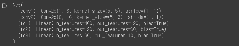
- 인풋 데이터 생성
- 파이토치에서 입력 데이터에는 반드시 배치 차원이 포함되어야 한다.
input = torch.randn(1, 1, 32, 32) # [batch size, 입력 채널 크기, 가로 길이, 세로 길이]
out = net(input)
print("out shape:", out.shape)
print(out)  # out shape: (1, 10)
# out shape: torch.Size([1, 10])
# tensor([[ 0.0300,  0.0742, -0.0155,  0.0461, -0.0405,  0.0761,  0.0242, -0.1358,
#          -0.0202, -0.1199]], grad_fn=<AddmmBackward0>)
- 정답으로 사용할 값을 임의로 만들어준다. 신경망의 출력 결과의 (1, 10)의 형태에 맞게 바꿔주어야 한다.
- view() 함수로 텐서를 reshape 해준다. (변경 전과 후의 원소 개수는 유지되어야 한다.)
- view(1, -1) : 첫번째 차원은 1이 되도록, -1로 표시된 2번째 차원은 파이토치가 알아서 계산
output = net(input)               # 입력 데이터를 신경망 모델에 전달하여 예측값을 얻음 shape: (1, 10)
print("output shape:", output.shape)
target = torch.randn(10)          # 임의의 텐서를 생성하여 정답값으로 가정
print ("target shape:", target.shape)
target = target.view(1, -1)       # 모델의 출력 텐서와 동일한 shape로 변경 : (1, 10)
print ("after reshape(view) -> target shape:", target.shape)

# output shape: torch.Size([1, 10])
# target shape: torch.Size([10])
# after reshape(view) -> target shape: torch.Size([1, 10])
[ 손실함수(Loss Function) 설정 ]
- 텐서의 requires_grad=True 옵션을 적용해주면 텐서에 실행되는 모든 연산들을 트래킹해서 자동으로 backpropagation을 수행해준다.
- 손실함수로 MSE를 설정해서 임의로 생성한 input과 target의 오차를 계산해보자. ( nn.MSELoss() 객체 생성)
### 손실함수 사용 예시
import torch
import torch.nn as nn

input = torch.randn(3, 5, requires_grad=True)
target = torch.randn(3, 5)

# MSE 객체 생성
criterion = nn.MSELoss()
output = criterion(input, target) # Loss 계산
output.backward()
print('input: ', input)
print('target: ', target)
print('output: ', output)

# input:  tensor([[ 0.1043, -0.4887, -0.6128, -0.4816, -0.8149],
#         [-0.9318,  0.6722,  0.9473,  0.3738, -2.6592],
#         [-1.8460, -1.4240,  0.3057,  1.2281, -0.4938]], requires_grad=True)
# target:  tensor([[-0.2818,  0.5413,  1.0230,  1.2985,  0.3693],
#         [-0.1413, -1.2815, -1.1806,  1.3397,  0.7307],
#        [ 1.4916, -0.5810, -1.2264, -1.1281,  0.8314]])
# output:  tensor(3.4237, grad_fn=<MseLossBackward0>)
[ 옵티마이저(Optimizer) 설정 ]
- torch.optim : 신경망 학습을 위한 파라미터 최적화 알고리즘이 구현되어 있는 클래스
- 모델의 학습 가능한 매개변수들은 모델.parameters()에 의해 반환된다.
- 파이토치에서는 backward 할 때 gradient 값들을계속 누적하기 때문에 학습을 시작하기 전에 gradient 버퍼를 zero로 리셋해주어야 한다. ( optimizer.zero_grad() )
- 앞에서 설명된 내용을 기반으로 학습을 수행하는 코드를 작성했다.
- backward()를 수행한 뒤에는 optimizer.step()으로 실제 파라미터를 갱신된 값으로 업데이트 해준다.
import torch.optim as optim

# Adam Optimizer 객체 생성, 모델의 학습시킬 파라미터 전달, 학습률 설정
optimizer = optim.Adam(net.parameters(), lr=0.01)

# 학습 과정(training loop)
optimizer.zero_grad()

input = torch.randn(1, 1, 32, 32)
output = net(input)
target = torch.randn(10)          # 예시를 위한 임의의 정답
target = target.view(1, -1)       # 출력과 같은 shape로 만듬
loss = criterion(output, target)  # Loss 계산
print(loss)

loss.backward()         # 역전파 함수 실행을 통해 gradient 계산
optimizer.step()        # gradient를 기반으로 실제 파라미터 업데이트를 실행

# tensor(1.1583, grad_fn=<MseLossBackward0>)
[ GPU 가속 이용하기 ]
- GPU 가속 가능 여부 확인
# 현재 개발환경에서 GPU 가속이 가능한지 확인
print(torch.cuda.is_available())
# GPU 연결되어 있으면 True, 아니면 False
- 디바이스 설정
# GPU 사용이 가능하면 cuda로 연산하도록 device를 설정 그렇지 않으면 cpu로 설정
device = torch.device("cuda" if torch.cuda.is_available() else "cpu")

# 신경망 모델에 디바이스 설정
net.to(device)
# Net(
#   (conv1): Conv2d(1, 6, kernel_size=(5, 5), stride=(1, 1))
#   (conv2): Conv2d(6, 16, kernel_size=(5, 5), stride=(1, 1))
#   (fc1): Linear(in_features=400, out_features=120, bias=True)
#   (fc2): Linear(in_features=120, out_features=60, bias=True)
#   (fc3): Linear(in_features=60, out_features=10, bias=True)
# )
- 랜덤한 학습 데이터 생성
train_inputs = torch.randn(100, 32, 128) # [전체 데이터 개수, 데이터의 최대 길이, 히든 벡터 크기]
train_labels = torch.randn(100, 3) # [전체 데이터 개수, 예측할 클래스 개수]
[ TensorDataset, DataLoader, RandomSampler, SequentialSampler ]
: 데이터셋을 샘플링하고, 학습 루프를 편리하게 구현하기 위한 함수
torch.utils.data에서 임포트 해준다.
# Dataset에 필요한 패키지 임포트
from torch.utils.data import TensorDataset, DataLoader, RandomSampler, SequentialSampler
미니배치 사이즈 만큼 매 학습 step마다 샘플링 해주도록 데이터셋을 구성
- TensorDataset() : 학습데이터와 레이블을 하나의 TensorDataset으로 결합 가능
- SequentialSampler(), RandomSampler() : 데이터를 샘플링 할 함수(순차적으로 뽑아올지, 랜덤하게 뽑아올지)
- DataLoader() : 미니배치 단위로 데이터를 자동 로딩
batch_size = 12 # 매 학습 Step 마다 샘플링할 데이터 개수

train_data = TensorDataset(train_inputs, train_labels)
train_sampler = RandomSampler(train_data)
train_dataloader = DataLoader(train_data, sampler=train_sampler, batch_size=batch_size)
- dataloader를 사용해서 학습 루프 생성
# dataloader를 통해서 학습 루프 생성
for step, batch in enumerate(train_dataloader): # enumerate : 인덱스(index)와 데이터값에 동시에 접근
  x_data, x_label = batch # batch_size=12개 만큼 데이터를 로딩
  # 데이터 로딩 step
  print(step, x_data.shape, x_label.shape)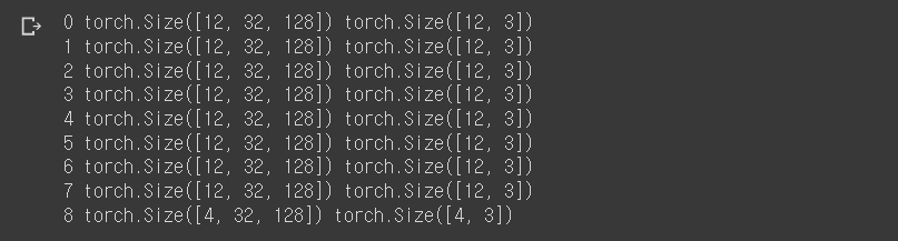
728x90
반응형
'인공지능 AI' 카테고리의 다른 글
| 모델 저장 및 불러오기 - Joblib, keras (0) | 2022.11.18 |
|---|---|
| [ ImageDataGenerator, ModelCheckpoint ] (0) | 2022.09.26 |
| [ OpenCV로 동영상 불러오기, glob ] (0) | 2022.09.26 |
| [ LightGBM ] (0) | 2022.09.11 |
| [ 정규화 : RobustScaler ] (0) | 2022.09.10 |